Ping Pong Ball Target System

Figure 1, Ping Pong Robot

Member Names (with emails)

KoTung Lin (kevinlin [at] umich.edu)

Daniel Cheng (udx [at] umich.edu)

Brief Project Description

Our goal is to implement the the inverse kinematic and forward kinematic for the ping pong ball robot and make the ping pong reaching the entire workspace. We will attempt to achieve the following: ground target aiming, trajectory planning for singularity prevention and integrate with the GUI operation panel for with trajectory prediction.

Objectives

• Forward kinematic
• Inverse kinematic
• Singularity prevention
• Graphic User Interface
• Trajectory prediction and projection to the alternative camera view point

Picture

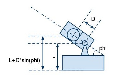Figure 2, Parameter of Robot

Figure 3, Parameter of robot for the taskspace

Figure 4, Taskspace

Figure 5, Coordinate of the operator

 

Model, including Jacobian

Forward Kinematic

If the operator provides input variable with theta and phi. We should able to use the forward kinematic to predict the entire ball trajectory.


Base on Newton's law of motion,

Considering only the vertical motion, we have

By rearrangement of terms, the equation becomes

and the solution of flight time is

After we solved for flight time, the shooting range of ball will be

 

Finally, the location of ball were the ball falls are

Inverse Kinematic

By providing the desired loaction [x, y] we compute the corresponding phi and theta. Since we do the computation under cylindrical coordinates, the first step would be coordinate transformation.

  

After transformation of coordinates, we could integrate the differential Jacobian to compute the two desired angles.

Jacobian Matrix
 
Consider the system without the wind resistance and friction, under the cylindrical coordinates, the flight range would be

The first term is the product of velocity and flight time, which give us the distance of ping pong ball travels before hitting the ground. The second term represents the initial movement after the barrel is moved.


By differentiation, the flying range of ping pong ball (r) to the angle Phi, we could get the differential relation

The only thing really which needs to computed here is the shooting range of ping pong versus the angle of barrel (phi).

First, we already compute the time of ping pong flight time by forward kinematic, which is

After that, based on flight time, we could have the differential relation range of ping pong ball versus phi

 

and all the entries of Jacobian matrix are known.

Now, we have the Jacobian Matrix for computing the inverse kinematic problem. By repeated integration of [ d phi/dt , d theta/dt ], we could have the angle phi and theta corresponded with the location [x, y].

Block Diagram

Figure 6, Inverse Kinematic Computation

Control Design

Since we use Euler method to compute the integral of state, the error for each time computation will accumulate into a large number (Figure 7). The strategy is to use a simple K controller to perform the contraction mapping. By differentiation of the Lyapunov function, the state will eventually converge to a equilibrium, so we could have a accurate angle. 

Figure 7, Error of Euler Method

Figure 8, joint variable after converging progress

Figure 9, simulation of trajectory with input location [-5, 5]

We also use the condition number of the Jacobian matrix to verify the case when the matrix is "almost" not invertible. By checking the ratio of maximum and minimum singular value of Jacobian, we could know when the inverse kinematic is unavailable to solve. We decide the condition number 300 will be good enough to prevent the singularity problem.

However, if we switch to the damped least square Jacobian matrix, the original converging process will be a problem. The damped least square Jacobian matrix try to drive the state out of singularity, but the converging progress will drive the state to approach singularity. Eventually, the state will become unstable and causing oscillation. 


How to prevent this from happening?  The ping pong ball robot has a property of redundancy for each target spot (barrel up/down), so we don't actually need to go through the singularity position for solving the differential kinematic. The only purpose for this implementation is for the scenario when target spot is far away from the taskspace. Under this situation, we simply turn off the feedback loop and use the solution from damped least square. Since the ping pong ball robot have only two joints, and the angle of bearing could be directly obtained from the input [x,y]. Therefore, the only variable left for damped least square method is r, and it will generate a nearest solution for robot to aim.

Figure 10, Damped Least Square Method with a location out of range [-10,10]

Figure 11, trajectory simulation with a location out of range [-10,10]

Implementation Notes

The overall structure of our robot is using arduino UNO to drive the ping pong ball robot and integrate with the MATLAB to perform the control.

 

GUI Interface 

The GUI interface is designed to implement forward (FK) and inverse (IK) kinematics with ease. The parameters for FK could be entered via text boxes or scroll bar below the 'Plot Theta/Phi' push button. To implement IK, values are entered below the 'Plot XY' push button. To execute FK or IK after value entry, the 'Plot Theta/Phi' and 'Plot XY' buttons are pressed respectively. When values for FK are provided and executed the corresponding XY values would be displayed in the text entry boxes, likewise when XY values are enter for IK the corresponding forward kinematic values of Theta/Phi are calculated and displayed on the entry boxes.

The previous trajectory path are overwritten by new plots. Trajectories could also be manually cleared by 'Clear Plots' push button.

The GUI is design to display the trajectory path of the projectile in the 3rd person perspective behind the pingpong cannon. An background image of the pingpong cannon's testing environment is added to show relative accuracy of the trajectory prediction in a live setting. The Theta and Phi angle therefore correspond to the left/right and up/angles of the barrel aim respectively.

Before initializing the GUI, a background image file would have to be present in the MATLAB code execution coder with corresponding name as the image reader name. When MATLAB code is executed, the image should appear on the plot space area. In order to view the trajectory clearly especially under complex background image conditions, the image could be changed to gray scale or the lines of trajectory could be made thicker.

Note: There is both angle and XY value limitations due to the physical performance of the cannon's actuating servos and solenoid power. The hard limits of Theta/Phi angles are shown at the side of the scroll bars. If values outside the allowable values are entered, the values would be changed to the closest permissible value. The limit for XY values are scaled to 10.

Trajectory  Prediction

The trajectory prediction on a 3rd person perspective, is implement by the homogeneous coordinate.

Figure 12, homogeneous coordinate (source from wikipedia)

Use the homogeneous transform, and change the trajectory coordinate to the coordinate of camera. After that, apply the formula of projection, and eliminate the information of principle axis. We could have the trajectory from the 3rd person view point.

Figure 13, formula of the coordinate projection

The right hand side capital [X, Y, Z] are the coordinate under homogeneous coordinate (figure 12). The [x', y'] of left hand side is the coordinate on the picture. K matrix represent the intrinsic parameter of camera, and g matrix is the homogeneous transformation of camera. From the figure 14, the thick yellow line will be the corresponding trajectory.

Figure 14, plot the prediction trajectory to on the picture

Results (Video)